

Paper Info#
| Item | Details |
|---|---|
| Venue | 2021 10th International Congress on Advanced Applied Informatics (IIAI-AAI) |
| Authors | Wei-Yi Chung, Yen-Nan Ho, Yu-Hsuan Wu, Jheng-Long Wu |
| DOI | 10.1109/IIAI-AAI53430.2021.00070 |
| Code | h30306/A-Dynamic-Embedding-Method-for-Passenger-Flow-Estimation |
| Slides | Conference_Howard_20210706.pdf |
| Award | Competitive Paper Award |
This was the first paper from our MRT traffic project. As first author I designed the model, ran the experiments, wrote the paper, and presented it in English at the online conference. The extended journal version was later published in Knowledge-Based Systems; see Dynamic Traffic Network Representation Model.
In one sentence: take the NLP pre-training recipe and apply it to MRT passenger flow. BERT first learns station distances and flow dynamics from pairs of station flow sequences; its dynamic station embeddings then replace the fixed Node2Vec vectors inside GMAN. Transfer-station MAE drops from 1.47 to 0.93.
Motivation#
Why traffic prediction uses embeddings#
Passenger flow depends on many factors (time of day, station location, neighbouring stations, transfer relations), and the data are imbalanced: flow is steady most of the time and peaks are short. Feeding raw features straight into a model often works poorly, so recent work first compresses the traffic state into a high-dimensional embedding and hands that to a downstream model:
- Tensor decomposition embeds multi-way traffic patterns, improving RMSE by about 20%.
- A graph embedding RNN (GERNN) represents the road network inside a traffic prediction framework.
Transfer learning for traffic#
Since embeddings help, the natural next step is pre-train, then transfer: pre-train on a traffic-related objective so the model understands traffic characteristics, then move it to the downstream task. For example:
- Pre-training on human trajectory data with a CBOW framework, transferred to three location-based prediction tasks.
- Pre-training accident-information embeddings combined with CNN and LSTM for highway traffic prediction.
The problem with static embeddings#
All of these share one trait: after transfer, each station (or location) maps to a single fixed vector. Traffic varies a lot, though; a station at peak hours on a weekday is in a completely different state from the same station on a quiet weekend. Fixed vectors lack diversity, which makes complex patterns hard to learn. Work on “dynamic features” at the time mostly focused on dynamic graph embeddings; nobody had used pre-training to produce dynamic station embeddings.
Why attention#
A second thread is the success of attention in traffic prediction. ASTGCN, for example, uses spatio-temporal attention to capture dynamic correlations and beats its baselines on two PeMS datasets. Attention weights inputs by importance, so it can pick out the spatial features that matter most for a target station, and unlike an RNN it parallelises.
Putting these together, the idea here is to generate station embeddings with attention-based BERT, and to make them change with the current passenger flow. GMAN was chosen as the downstream model because it is attention-based itself and has a clearly separable Spatial Embedding (SE) to swap out.
Problem Definition#
Given a station’s hourly flow over the past P hours, X' = (x'_1, …, x'_P), predict the next hour’s flow y_NTF = x'_{P+1} (NTF = next time step flow).
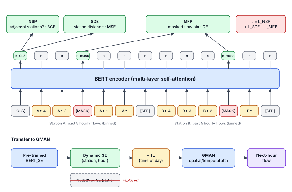
The pipeline has two stages: pre-train BERT_SE, then plug it into GMAN and train for flow prediction.
Stage 1: Pre-training BERT_SE#
Input construction#
Each training example takes two MRT stations a and b over the same time window, each with its last 5 hourly flows:
X_t^S = (x_{t-4}^S, x_{t-3}^S, x_{t-2}^S, x_{t-1}^S, x_t^S)
H_out = BERT_SE(concat[X_t^a, X_t^b])
Flow is continuous and hard to predict directly, so it is first binned into categories, turning each hour into a token, like a word. The two sequences are joined in BERT format:
[CLS] a(t-4) a(t-3) a(t-2) a(t-1) a(t) [SEP] b(t-4) b(t-3) b(t-2) b(t-1) b(t) [SEP]
BERT’s standard random masking is applied. Through multiple self-attention layers the two stations’ flows attend to each other, giving a hidden state per position, H_out = [h_1, h_2, …, h_10].
Objectives#
The paper formally describes two self-supervised objectives, trained jointly:
SDE (Station Distance Estimation)
From BERT’s point of view, the most obvious relation between the two sequences is how far apart their stations are. The [CLS] output predicts the straight-line distance between the two stations:
ŷ_SDE = W_SDE · h_1 + b_SDE
l_SDE = (y_SDE − ŷ_SDE)²
This teaches the model the spatial relationship between stations.
MFP (Masked Flow Prediction)
Predict which flow bin each masked hour falls into, so the model learns how flow changes across the sequence:
h_i^FP = LayerNorm(GELU(W_FP1 · h_i + b_FP1))
ŷ_FP  = W_FP2 · h_i^FP + b_FP2
l_FP  = −(1/N) Σ y_FP · log(ŷ_FP)
The head has the same structure as BERT’s original MLM head.
Total loss is the plain sum, L(θ_SE) = l_SDE + l_FP, optimised with Adam.
A third objective in the code: the repo folder is called BERT_three_loss because the implementation keeps an NSP-style head as well. It is not BERT’s next-sentence prediction; it predicts whether stations a and b are adjacent on the line. Data_preparing_threeloss.py holds an adjacency table for every station (adjacent = 1, otherwise 0), and the head uses BCE loss. The total loss in the code is masked_lm_loss + loss_NSP + loss_Dist.
Why the embedding is “dynamic”#
The input itself is a specific station’s flow over a specific window. The same station sends different sequences at peak and off-peak hours, so BERT’s output vector naturally differs. SDE (and the adjacency head in the code) gives the vector spatial information, while MFP gives it information about how flow evolves over time.
Stage 2: Transfer to GMAN#
What GMAN is#
GMAN (Graph Multi-Attention Network) is an encoder-decoder made of:
| Component | Role |
|---|---|
| STAttBlock | Spatio-temporal attention block, attending over the spatial and temporal dimensions |
| TransAtt | Transform attention that maps encoder (historical) steps to decoder (future) steps |
| FC × 2 | Fully-connected layers at the input and output |
| STE | Spatio-temporal embedding = SE (Spatial Embedding, geography) + TE (Temporal Embedding, time) |
GMAN’s original SE is computed with Node2Vec on the network graph, so a station always has the same vector and cannot adapt to the current flow.
Swapping the SE#
Only the SE changes. The historical flow x'_p goes into the pre-trained BERT_SE to get each station’s dynamic vector, and those vectors form the SE for the whole graph:
se_p = BERT_SE(x'_p)
SE   = (se_1, se_2, …, se_N)        # N = number of stations
ŷ_NTF = GMAN(X', BERT_SE)
TE and the rest of GMAN follow the original paper. GMAN is trained on MAE between predicted and actual flow, L(θ_GMAN) = |y_NTF − ŷ_NTF|, also with Adam.
Experimental Setup#
Data#
Hourly entry/exit flows of the Taipei MRT from January 2017 to March 2019. Stations are split into transfer and non-transfer stations depending on whether lines intersect there, with 10 of each, 20 in total. All flows are log-normalised to reduce scale differences between stations.
| Raw data statistics (Table I) | Transfer | Non-transfer |
|---|---|---|
| Max flow | 10,566 | 46,225 |
| Min flow | 0 | 0 |
| Mean flow | 1,167 | 4,532 |
| Std. dev. | 1,356 | 5,329 |
| Examples | 172,710 | 172,710 |
Splits#
Split by time to avoid leaking future information:
| Set | Period |
|---|---|
| Train | 2017/01 – 2018/09 |
| Validation | 2018/09 – 2018/12 |
| Test | 2019/01 – 2019/03 |
All results below are on the test set.
Hyperparameters (Table II)#
| Parameter | Value | Meaning |
|---|---|---|
| hp | 1, 3, 5 | Number of historical time steps fed to GMAN |
| fs | 1500, 2000, None | Filter neighbouring stations by distance (metres); None uses every station |
| lr | 1e-4 | Learning rate |
| es | 64 | BERT embedding size, also GMAN’s hidden size |
Other GMAN parameters follow the original paper, and BERT’s architecture parameters follow the original BERT.
Distance filtering keeps only stations near the target, cutting noise from unrelated stations. After filtering, every station has at least one neighbour within both 1500 m and 2000 m, with 6.5 and 9.5 neighbours on average respectively. Stations with more neighbours are more likely to be transfer stations or close to the city centre.
Baselines and metrics#
- node2vec_SE: original GMAN, static station embedding.
- BERT_SE: this paper, dynamic station embedding.
- Metrics: MAE and RMSE, the two standard regression metrics.
Results#
1. Static vs dynamic embedding (Table III)#
| Spatial embedding | Transfer MAE | Non-transfer MAE |
|---|---|---|
| node2vec_SE | 1.47 | 1.23 |
| BERT_SE | 0.93 | 1.24 |
- Transfer stations improve a lot: MAE falls from 1.47 to 0.93. Transfer stations carry peak flow and are where congestion happens, so accuracy there has the most practical impact.
- Non-transfer stations are essentially flat: BERT_SE is 0.01 behind.
Note: in the published Table III the RMSE column is smaller than MAE, which is impossible (RMSE ≥ MAE always), so the columns were likely garbled during typesetting; only MAE is listed here. The text also says transfer MAE is “0.97” while the table says 0.93; this post follows the table.
2. History length (Table IV)#
| History steps hp | BERT_SE MAE | BERT_SE RMSE | node2vec_SE MAE | node2vec_SE RMSE |
|---|---|---|---|---|
| 1 | 0.85 | 1.51 | 2.05 | 2.94 |
| 3 | 2.56 | 3.64 | 1.69 | 2.17 |
| 5 | 1.97 | 2.86 | 1.57 | 1.99 |
The two embeddings trend in opposite directions:
- BERT_SE is best with a single step (MAE 0.85). The paper’s explanation is that the most informative signal for the next hour is the previous hour. My reading is that the dynamic embedding already carries recent flow from BERT’s 5-hour input, so extra GMAN steps add nothing.
- node2vec_SE improves with more history (2.05 → 1.69 → 1.57). With a fixed SE, the model can only make up the information through longer flow history, which matches GMAN’s design.
3. Filtering neighbouring stations by distance (Table V)#
| Filter fs | BERT_SE MAE | BERT_SE RMSE | node2vec_SE MAE | node2vec_SE RMSE |
|---|---|---|---|---|
| None | 1.46 | 2.04 | 1.21 | 1.80 |
| 1500 m | 0.83 | 1.50 | 1.18 | 1.59 |
| 2000 m | 0.83 | 1.50 | 1.19 | 1.61 |
- Both embeddings improve with filtering, BERT_SE dramatically (1.46 → 0.83). A station’s flow is mainly influenced by nearby stations; using every station does not help and makes training much slower.
- 1500 m and 2000 m give identical results for BERT_SE; for node2vec_SE 1500 m is slightly better.
- Without filtering (None), node2vec_SE actually beats BERT_SE. The advantage of dynamic embeddings only shows up with a sensible neighbourhood.
Conclusion and Limitations#
Conclusion: dynamic embeddings from BERT_SE improve GMAN’s MRT flow prediction overall, especially at transfer stations, showing that the diversity of dynamic embeddings represents station state better than static ones. Multi-objective pre-training also lets the model learn more facets of traffic.
Limitations, looking back at my own paper:
- Only 20 stations, a small scale.
- The gain is concentrated at transfer stations; non-transfer stations do not improve.
- BERT_SE gets clearly worse at hp=3 (MAE 2.56). The trend is not monotonic, and the paper does not analyse why.
- The paper’s future work proposes new pre-training objectives, such as next-station prediction, to give the embedding a better understanding of traffic.
The journal version continues this line: four pre-training objectives (MFP, same route, adjacent station, station distance) and a downstream hierarchical attention model over time, stations and routes. See Dynamic Traffic Network Representation Model.
Code and Resources#
The GitHub repo contains:
Project/data/: station info, distance matrix, and sample 2019 flow data (raw 2017 and 2018 data are not included)Project/model/Data_preparing_threeloss.py: builds pre-training data (paired station sequences, distance, adjacency)Project/model/BERT_three_loss/: BERT_SE pre-training (run_train.sh) and embedding export (predict_embeddings.py)- Downstream prediction reuses GMAN; just replace SE with BERT’s output
My local folder also keeps every submission version (BERTSE_2021xxxx), a Chinese draft of the paper, the talk script and the acceptance notice.